Z Transform and Its Properties From DTFT, we have,
x [ t ] = 1 2 π ∫ − π + π X ( ω ) e j ω t d ω X ( ω ) = ∑ − ∞ + ∞ x [ t ] e − j ω t x[t] = \frac{1}{2\pi} \int_{-\pi}^{+\pi} X(\omega) e^{j \omega t} \mathrm{d} \omega \\
X(\omega) = \sum_{-\infty}^{+\infty} x[t] e^{-j \omega t} x [ t ] = 2 π 1 ∫ − π + π X ( ω ) e jω t d ω X ( ω ) = − ∞ ∑ + ∞ x [ t ] e − jω t Again, we multiply the kernel with a real exponential, just like Laplace Transform (z transform is a discrete version of Laplace Transform). We note, z = e j ω + σ z = e^{j \omega + \sigma} z = e jω + σ
X ( z ) = ∑ t = − ∞ + ∞ x [ t ] z − t X(z) = \sum_{t = -\infty}^{+\infty} x[t] z^{-t} X ( z ) = t = − ∞ ∑ + ∞ x [ t ] z − t If we would like X ( z ) X(z) X ( z )
lim t → + ∞ ∣ x [ t + 1 ] z − ( t + 1 ) x [ t ] z − t ∣ < 1 \lim_{t \to +\infty} |\frac{x[t + 1] z^{-(t + 1)}}{x[t] z^{-t}}| < 1 t → + ∞ lim ∣ x [ t ] z − t x [ t + 1 ] z − ( t + 1 ) ∣ < 1 Which is equivalent to,
∣ z ∣ > lim t → + ∞ x [ t ] x [ t + 1 ] |z| > \lim_{t \to +\infty} \frac{x[t]}{x[t + 1]} ∣ z ∣ > t → + ∞ lim x [ t + 1 ] x [ t ] And vice versa on the negative side.
∣ z ∣ < lim t → − ∞ x [ t ] x [ t − 1 ] |z| < \lim_{t \to -\infty} \frac{x[t]}{x[t - 1]} ∣ z ∣ < t → − ∞ lim x [ t − 1 ] x [ t ] For certain points that,
∣ z ∣ = lim t → + ∞ x [ t ] x [ t + 1 ] |z| = \lim_{t \to +\infty} \frac{x[t]}{x[t + 1]} ∣ z ∣ = t → + ∞ lim x [ t + 1 ] x [ t ] Wether the series will converge depends on the phase of z z z
And vice versa for the negative side.
And technically,
x [ t ] = − j 1 2 π ∫ − j π + σ + j π + σ X ( z ) z t d ( j ω + σ ) = 1 2 π j ∫ e − j π + σ e + j π + σ X ( z ) z t − 1 d z x[t] = -j \frac{1}{2\pi} \int_{-j \pi + \sigma}^{+j\pi + \sigma} X(z) z^t \mathrm{d} (j \omega + \sigma) \\
= \frac{1}{2\pi j} \int_{e^{-j \pi + \sigma}}^{e^{+j\pi + \sigma}} X(z) z^{t - 1} \mathrm{d}z x [ t ] = − j 2 π 1 ∫ − jπ + σ + jπ + σ X ( z ) z t d ( jω + σ ) = 2 πj 1 ∫ e − jπ + σ e + jπ + σ X ( z ) z t − 1 d z But, wait, e − j π + σ = e + j π + σ e^{-j \pi + \sigma} = e^{+j\pi + \sigma} e − jπ + σ = e + jπ + σ
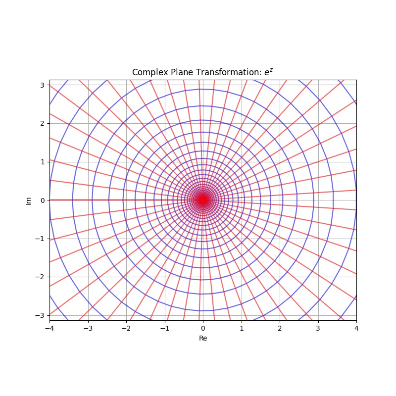
Let's consider e j x + σ e^{jx + \sigma} e j x + σ x x x − π -\pi − π π \pi π e σ e^\sigma e σ
In the picture, that is starting from a point, walking alongside the blue line (the old line that was parallel to the real line before the transformation). A round is 2 π 2\pi 2 π x x x
That is to say,
x [ t ] = 1 2 π j ∮ C ( e σ ) X ( z ) z t − 1 d z x[t] = \frac{1}{2\pi j} \oint_{C(e^\sigma)} X(z) z^{t - 1} \mathrm{d}z x [ t ] = 2 πj 1 ∮ C ( e σ ) X ( z ) z t − 1 d z And C ( e σ ) C(e^\sigma) C ( e σ ) e σ e^\sigma e σ σ \sigma σ
For convenience, if we write C C C
There is another way to directly get the inverse z transform, because,
X ( z ) = ∑ t = − ∞ + ∞ x [ t ] z − t X(z) = \sum_{t = -\infty}^{+\infty} x[t] z^{-t} X ( z ) = t = − ∞ ∑ + ∞ x [ t ] z − t Based on the Cauchy Integral, that,
∮ P f ( z ) ( z − z 0 ) n d z = 2 π j f ( n − 1 ) ( z 0 ) n ! Where f ( z ) is continuous within P and P is any curve that contains z 0 \oint_{P} \frac{f(z)}{(z-z_0)^n} \mathrm{d}z = 2\pi j \frac{f^{(n - 1)}(z_0)}{n!} \\
\text{Where} \quad f(z) \text{ is continuous within } P \text{ and } P \text{ is any curve that contains } z_0 ∮ P ( z − z 0 ) n f ( z ) d z = 2 πj n ! f ( n − 1 ) ( z 0 ) Where f ( z ) is continuous within P and P is any curve that contains z 0 So if we want x [ t ] x[t] x [ t ]
X ( z ) z t − 1 = ∑ k = − ∞ + ∞ x [ k ] z − k + t − 1 X(z) z^{t - 1} = \sum_{k = -\infty}^{+\infty} x[k] z^{-k + t - 1} X ( z ) z t − 1 = k = − ∞ ∑ + ∞ x [ k ] z − k + t − 1 Thus,
∮ C ( r ) X ( z ) z t − 1 d z = 2 π j x [ t ] \oint_{C(r)} X(z) z^{t-1} \mathrm{d}z = 2 \pi j x[t] ∮ C ( r ) X ( z ) z t − 1 d z = 2 πj x [ t ] X ( z ) X(z) X ( z ) C C C r r r
Similarly, we sometimes also use single side z transform. We don't usually care about the negative side.
So in conclusion,
The z transform is,
x [ t ] = 1 2 π j ∮ C ( e σ ) X ( z ) z t − 1 d z X ( z ) = ∑ t = − ∞ + ∞ x [ t ] z − t e σ 0 < ∣ z ∣ < e β 0 x[t] = \frac{1}{2\pi j} \oint_{C(e^\sigma)} X(z) z^{t - 1} \mathrm{d}z \\
X(z) = \sum_{t = -\infty}^{+\infty} x[t] z^{-t} \quad e^{\sigma_0} < |z| < e^{\beta_0} x [ t ] = 2 πj 1 ∮ C ( e σ ) X ( z ) z t − 1 d z X ( z ) = t = − ∞ ∑ + ∞ x [ t ] z − t e σ 0 < ∣ z ∣ < e β 0 The single side z transform is,
x [ t ] = 1 2 π j ∮ C ( e σ ) X ( z ) z t − 1 d z X ( z ) = ∑ t = 0 + ∞ x [ t ] z − t ∣ z ∣ > e σ 0 x[t] = \frac{1}{2\pi j} \oint_{C(e^\sigma)} X(z) z^{t - 1} \mathrm{d}z \\
X(z) = \sum_{t = 0}^{+\infty} x[t] z^{-t} \quad |z| > e^{\sigma_0} x [ t ] = 2 πj 1 ∮ C ( e σ ) X ( z ) z t − 1 d z X ( z ) = t = 0 ∑ + ∞ x [ t ] z − t ∣ z ∣ > e σ 0 We note the pair as,
x ( t ) → ± Z X ( z ) ∣ z ∣ > e σ 0 x(t) \xrightarrow{\pm \mathcal{Z}} X(z) \quad |z| > e^{\sigma_0} x ( t ) ± Z X ( z ) ∣ z ∣ > e σ 0 And the single side pair as,
x ( t ) → Z X ( z ) e σ 0 < ∣ z ∣ < e β 0 x(t) \xrightarrow{\mathcal{Z}} X(z) \quad e^{\sigma_0} < |z| < e^{\beta_0} x ( t ) Z X ( z ) e σ 0 < ∣ z ∣ < e β 0 Properties
Linearity
a x [ t ] + b y [ t ] → Z a X ( z ) + b Y ( z ) ∣ z ∣ > max ( e σ 0 , e σ 1 ) a x[t] + b y[t] \xrightarrow{\mathcal{Z}} a X(z) + b Y(z) \quad |z| > \max(e^{\sigma_0}, e^{\sigma_1}) a x [ t ] + b y [ t ] Z a X ( z ) + bY ( z ) ∣ z ∣ > max ( e σ 0 , e σ 1 ) a x [ t ] + b y [ t ] → ± Z a X ( z ) + b Y ( z ) max ( e σ 0 , e σ 1 ) < ∣ z ∣ < min ( e β 0 , e β 1 ) a x[t] + b y[t] \xrightarrow{\pm \mathcal{Z}} a X(z) + b Y(z) \quad \max(e^{\sigma_0}, e^{\sigma_1}) < |z| < \min(e^{\beta_0}, e^{\beta_1}) a x [ t ] + b y [ t ] ± Z a X ( z ) + bY ( z ) max ( e σ 0 , e σ 1 ) < ∣ z ∣ < min ( e β 0 , e β 1 ) Shifting Time is Shifting Phase
We need to distinguish three cases when we consider time shifting.
Two sides z transform
Single side z transform on casual signals
Single side z transform on non-casual signals
Previously in the Laplace Transform, we only talked about single side transform on casual signals, because time shifting isn't very important in practice of Laplace Transform. However, since difference equation utilizes shifting, it's crucial to consider all off the three cases.
Again, in the following sections, if we don't say otherwise, the region of convergence won't change.
Suppose,
x [ t ] → ± Z X ( z ) x[t] \xrightarrow{\pm \mathcal{Z}} X(z) x [ t ] ± Z X ( z ) We have,
∑ t = − ∞ + ∞ x [ t + t 0 ] z − t = z t 0 ∑ t + t 0 = − ∞ + ∞ x [ t ] z − ( t + t 0 ) = z t 0 X ( z ) \sum_{t = -\infty}^{+\infty} x[t + t_0] z^{-t} \\
= z^{t_0} \sum_{t + t_0 = -\infty}^{+\infty} x[t] z^{- (t + t_0)} \\
= z^{t_0} X(z) t = − ∞ ∑ + ∞ x [ t + t 0 ] z − t = z t 0 t + t 0 = − ∞ ∑ + ∞ x [ t ] z − ( t + t 0 ) = z t 0 X ( z ) That's to say,
x [ t + t 0 ] → ± Z z t 0 X ( z ) x[t + t_0] \xrightarrow{\pm \mathcal{Z}} z^{t_0} X(z) x [ t + t 0 ] ± Z z t 0 X ( z ) Casual signals are signals that has value zero on the negative side. Thus,
x [ t ] u [ t ] → Z X ( z ) x[t]u[t] \xrightarrow{\mathcal{Z}} X(z) x [ t ] u [ t ] Z X ( z ) ∑ t = 0 + ∞ x [ t + t 0 ] u [ t + t 0 ] z − t = z t 0 ∑ t + t 0 = t 0 + ∞ x [ t + t 0 ] u [ t + t 0 ] z − ( t + t 0 ) = z t 0 ∑ + t + t 0 = 0 + ∞ x [ t + t 0 ] u [ t + t 0 ] z − ( t + t 0 ) = z t 0 X ( z ) \sum_{t = 0}^{+\infty} x[t + t_0] u[t + t_0] z^{-t} \\
= z^{t_0} \sum_{t + t_0 = t_0}^{+\infty} x[t + t_0] u[t + t_0] z^{-(t + t_0)} \\
= z^{t_0} \sum+{t + t_0 = 0}^{+\infty} x[t + t_0] u[t + t_0] z^{-(t + t_0)} \\
= z^{t_0} X(z) t = 0 ∑ + ∞ x [ t + t 0 ] u [ t + t 0 ] z − t = z t 0 t + t 0 = t 0 ∑ + ∞ x [ t + t 0 ] u [ t + t 0 ] z − ( t + t 0 ) = z t 0 ∑ + t + t 0 = 0 + ∞ x [ t + t 0 ] u [ t + t 0 ] z − ( t + t 0 ) = z t 0 X ( z ) That's to say,
x [ t + t 0 ] u [ t + t 0 ] → Z z t 0 X ( z ) x[t + t_0] u[t + t_0] \xrightarrow{\mathcal{Z}} z^{t_0} X(z) x [ t + t 0 ] u [ t + t 0 ] Z z t 0 X ( z ) Again,
x [ t ] → Z X ( z ) x[t] \xrightarrow{\mathcal{Z}} X(z) x [ t ] Z X ( z ) We need to distinct the shift towards the postive side and the shift towards the negative side. Thus, we assume t 0 ≥ 0 t_0 \geq 0 t 0 ≥ 0
For moving towards the negative side, the result is,
∑ t = 0 + ∞ x [ t + t 0 ] z − t = z t 0 ∑ t + t 0 = t 0 + ∞ x [ t + t 0 ] z − ( t + t 0 ) = z t 0 ( ∑ t + t 0 = 0 + ∞ x [ t + t 0 ] z − ( t + t ) − ∑ t + t 0 = 0 t 0 − 1 x [ t + t 0 ] z − ( t + t 0 ) ) = z t 0 X ( z ) − z t 0 ∑ t + t 0 = 0 t 0 − 1 x [ t + t 0 ] z − ( t + t 0 ) \sum_{t = 0}^{+\infty} x[t + t_0] z^{-t} \\
= z^{t_0} \sum_{t + t_0 = t_0}^{+\infty} x[t + t_0] z^{-(t + t_0)} \\
= z^{t_0} (\sum_{t + t_0 = 0}^{+\infty} x[t + t_0] z^{-(t + t)} - \sum_{t + t_0 = 0}^{t_0 - 1} x[t + t_0] z^{-(t + t_0)}) \\
= z^{t_0} X(z) - z^{t_0} \sum_{t + t_0 = 0}^{t_0 - 1} x[t + t_0] z^{-(t + t_0)} t = 0 ∑ + ∞ x [ t + t 0 ] z − t = z t 0 t + t 0 = t 0 ∑ + ∞ x [ t + t 0 ] z − ( t + t 0 ) = z t 0 ( t + t 0 = 0 ∑ + ∞ x [ t + t 0 ] z − ( t + t ) − t + t 0 = 0 ∑ t 0 − 1 x [ t + t 0 ] z − ( t + t 0 ) ) = z t 0 X ( z ) − z t 0 t + t 0 = 0 ∑ t 0 − 1 x [ t + t 0 ] z − ( t + t 0 ) Kind of ugly, to be honest.
For moving towards the positive side, the result is,
∑ t = 0 + ∞ x [ t − t 0 ] z − t = z − t 0 ∑ t − t 0 = − t 0 + ∞ x [ t − t 0 ] z − ( t − t 0 ) = z − t 0 ( ∑ t − t 0 = 0 + ∞ x [ t − t 0 ] z − ( t − t 0 ) + ∑ t − t 0 = − t 0 − 1 x [ t − t 0 ] z − ( t − t 0 ) ) = z − t 0 X ( z ) + z − t 0 ∑ t − t 0 = − t 0 − 1 x [ t − t 0 ] z − ( t − t 0 ) \sum_{t = 0}^{+\infty} x[t - t_0] z^{-t} \\
= z^{-t_0} \sum_{t - t_0 = -t_0}^{+\infty} x[t - t_0] z^{-(t - t_0)} \\
= z^{-t_0} (\sum_{t - t_0 = 0}^{+\infty} x[t - t_0] z^{-(t - t_0)} + \sum_{t - t_0 = -t_0}^{-1} x[t - t_0] z^{-(t - t_0)}) \\
= z^{-t_0} X(z) + z^{-t_0} \sum_{t - t_0 = -t_0}^{-1} x[t - t_0] z^{-(t - t_0)} t = 0 ∑ + ∞ x [ t − t 0 ] z − t = z − t 0 t − t 0 = − t 0 ∑ + ∞ x [ t − t 0 ] z − ( t − t 0 ) = z − t 0 ( t − t 0 = 0 ∑ + ∞ x [ t − t 0 ] z − ( t − t 0 ) + t − t 0 = − t 0 ∑ − 1 x [ t − t 0 ] z − ( t − t 0 ) ) = z − t 0 X ( z ) + z − t 0 t − t 0 = − t 0 ∑ − 1 x [ t − t 0 ] z − ( t − t 0 ) Well, just as ugly.
In conclusion, for t 0 ≥ 0 t_0 \geq 0 t 0 ≥ 0
x [ t − t 0 ] → Z z − t 0 X ( z ) + z − t 0 ∑ t − t 0 = − t 0 − 1 x [ t − t 0 ] z − ( t − t 0 ) x[t - t_0] \xrightarrow{\mathcal{Z}} z^{-t_0} X(z) + z^{-t_0} \sum_{t - t_0 = -t_0}^{-1} x[t - t_0] z^{-(t - t_0)} x [ t − t 0 ] Z z − t 0 X ( z ) + z − t 0 t − t 0 = − t 0 ∑ − 1 x [ t − t 0 ] z − ( t − t 0 ) x [ t + t 0 ] → Z z t 0 X ( z ) − z t 0 ∑ t + t 0 = 0 t 0 − 1 x [ t + t 0 ] z − ( t + t 0 ) x[t + t_0] \xrightarrow{\mathcal{Z}} z^{t_0} X(z) - z^{t_0} \sum_{t + t_0 = 0}^{t_0 - 1} x[t + t_0] z^{-(t + t_0)} x [ t + t 0 ] Z z t 0 X ( z ) − z t 0 t + t 0 = 0 ∑ t 0 − 1 x [ t + t 0 ] z − ( t + t 0 ) It's better that we simply memorize the case for pushing back 1 1 1 2 2 2
x [ t − 1 ] → Z z − 1 X ( z ) + x [ − 1 ] x [ t − 2 ] → Z z − 2 X ( z ) + x [ − 1 ] z − 1 + x [ − 2 ] x[t - 1] \xrightarrow{\mathcal{Z}} z^{-1} X(z) + x[-1] \\
x[t - 2] \xrightarrow{\mathcal{Z}} z^{-2} X(z) + x[-1] z^{-1} + x[-2] x [ t − 1 ] Z z − 1 X ( z ) + x [ − 1 ] x [ t − 2 ] Z z − 2 X ( z ) + x [ − 1 ] z − 1 + x [ − 2 ] For forwarding operators,
x [ t + 1 ] → Z z 1 X ( z ) − x [ 0 ] x [ t + 2 ] → Z z 2 X ( z ) − x [ 0 ] z 1 − x [ 1 ] z 2 x[t + 1] \xrightarrow{\mathcal{Z}} z^{1} X(z) - x[0] \\
x[t + 2] \xrightarrow{\mathcal{Z}} z^{2} X(z) - x[0] z^{1} - x[1] z^{2} x [ t + 1 ] Z z 1 X ( z ) − x [ 0 ] x [ t + 2 ] Z z 2 X ( z ) − x [ 0 ] z 1 − x [ 1 ] z 2 Z-Scale
x [ t ] → Z X ( z ) ∣ z ∣ < e σ 0 x[t] \xrightarrow{\mathcal{Z}} X(z) \quad |z| < e^{\sigma_0} x [ t ] Z X ( z ) ∣ z ∣ < e σ 0 ∑ t = − ∞ + ∞ x [ t ] a − t z − t = ∑ t = 0 + ∞ x [ t ] ( a z ) − t = X ( a z ) \sum_{t = -\infty}^{+\infty} x[t] a^{-t} z^{-t} \\
= \sum_{t = 0}^{+\infty} x[t] (az)^{-t} \\
= X(az) t = − ∞ ∑ + ∞ x [ t ] a − t z − t = t = 0 ∑ + ∞ x [ t ] ( a z ) − t = X ( a z ) a − t x [ t ] → Z X ( a z ) ∣ a z ∣ < e σ 0 a^{-t}x[t] \xrightarrow{\mathcal{Z}} X(az) \quad |az| < e^{\sigma_0} a − t x [ t ] Z X ( a z ) ∣ a z ∣ < e σ 0 Similarly,
a − t x [ t ] → ± Z X ( a z ) e σ 0 < ∣ a z ∣ < e β 0 a^{-t}x[t] \xrightarrow{\pm \mathcal{Z}} X(az) \quad e^{\sigma_0} < |az| < e^{\beta_0} a − t x [ t ] ± Z X ( a z ) e σ 0 < ∣ a z ∣ < e β 0 Z-Derivative
x [ t ] → Z X ( z ) x[t] \xrightarrow{\mathcal{Z}} X(z) x [ t ] Z X ( z ) That is,
X ( z ) = ∑ t = 0 + ∞ x [ t ] z − t X(z) = \sum_{t = 0}^{+\infty} x[t] z^{-t} X ( z ) = t = 0 ∑ + ∞ x [ t ] z − t Take derivative,
d X ( z ) d z = − ∑ t = 0 + ∞ t x [ t ] z − t − 1 \frac{\mathrm{d} X(z)}{\mathrm{d} z} = -\sum_{t = 0}^{+\infty} t x[t] z^{-t - 1} d z d X ( z ) = − t = 0 ∑ + ∞ t x [ t ] z − t − 1 − z d X ( z ) d z = ∑ t = 0 + ∞ t x [ t ] z − t -z \frac{\mathrm{d} X(z)}{\mathrm{d} z} = \sum_{t = 0}^{+\infty} t x[t] z^{-t} − z d z d X ( z ) = t = 0 ∑ + ∞ t x [ t ] z − t And thus,
t x [ t ] → Z − z d X ( z ) d z t x[t] \xrightarrow{\mathcal{Z}} -z \frac{\mathrm{d} X(z)}{\mathrm{d} z} t x [ t ] Z − z d z d X ( z ) It's identical to the two sides,
t x [ t ] → ± Z − z d X ( z ) d z t x[t] \xrightarrow{\pm \mathcal{Z}} -z \frac{\mathrm{d} X(z)}{\mathrm{d} z} t x [ t ] ± Z − z d z d X ( z ) Initial and Final Value Theorems
Suppose the sequence is right side- that is, there is an M M M
x [ t ] = 0 t < M x[t] = 0 \quad t < M x [ t ] = 0 t < M And,
X ( z ) = ∑ t = M + ∞ x [ t ] z − t X(z) = \sum_{t = M}^{+\infty} x[t] z^{-t} X ( z ) = t = M ∑ + ∞ x [ t ] z − t Thus,
lim z → + ∞ X ( z ) z M = lim z → + ∞ ∑ t = M + ∞ x [ t ] z − ( t − M ) = x [ M ] \lim_{z \to +\infty} X(z) z^{M} \\
= \lim_{z \to +\infty} \sum_{t = M}^{+\infty} x[t] z^{-(t - M)} \\
= x[M] z → + ∞ lim X ( z ) z M = z → + ∞ lim t = M ∑ + ∞ x [ t ] z − ( t − M ) = x [ M ] That is,
x [ M ] = lim z → + ∞ X ( z ) z M x[M] = \lim_{z \to +\infty} X(z) z^{M} x [ M ] = z → + ∞ lim X ( z ) z M For causal signals,
x [ 0 ] = lim z → + ∞ X ( z ) x[0] = \lim_{z \to +\infty} X(z) x [ 0 ] = z → + ∞ lim X ( z ) As for the final value theorem, consider,
X ( z ) = ∑ t = M + ∞ x [ t ] z − t X(z) = \sum_{t = M}^{+\infty} x[t] z^{-t} X ( z ) = t = M ∑ + ∞ x [ t ] z − t And,
lim z → 1 ( z − 1 ) X ( z ) = lim z → 1 ∑ t = M + ∞ x [ t ] ( z − t − z − ( t + 1 ) ) = lim z → 1 ∑ t = M + ∞ ( x [ t + 1 ] − x [ t ] ) z − t − x [ M ] z − M = x [ + ∞ ] \lim_{z \to 1} (z - 1) X(z) \\
= \lim_{z \to 1} \sum_{t = M}^{+\infty} x[t] (z^{-t} - z^{-(t + 1)}) \\
= \lim_{z \to 1} \sum_{t = M}^{+\infty} (x[t+1] - x[t]) z^{-t} - x[M] z^{-M} \\
= x[+\infty] z → 1 lim ( z − 1 ) X ( z ) = z → 1 lim t = M ∑ + ∞ x [ t ] ( z − t − z − ( t + 1 ) ) = z → 1 lim t = M ∑ + ∞ ( x [ t + 1 ] − x [ t ]) z − t − x [ M ] z − M = x [ + ∞ ] That is to say,
x [ + ∞ ] = lim z → 1 ( z − 1 ) X ( z ) x[+\infty] = \lim_{z \to 1} (z - 1) X(z) x [ + ∞ ] = z → 1 lim ( z − 1 ) X ( z ) This requires convergence condition of,
e σ < ∣ z ∣ e^{\sigma} < |z| e σ < ∣ z ∣ Where,
e σ < 1 e^{\sigma} < 1 e σ < 1 This is because we are approaching z z z
In conclusion,
The initial value theorem is,
x [ M ] = lim z → + ∞ X ( z ) z M x[M] = \lim_{z \to +\infty} X(z) z^{M} x [ M ] = z → + ∞ lim X ( z ) z M The final value theorem is,
x [ + ∞ ] = lim z → 1 ( z − 1 ) X ( z ) x[+\infty] = \lim_{z \to 1} (z - 1) X(z) x [ + ∞ ] = z → 1 lim ( z − 1 ) X ( z ) Convolution
Consider,
x [ t ] → Z X ( z ) e σ 0 < ∣ z ∣ y [ t ] → Z Y ( z ) e σ 1 < ∣ z ∣ x[t] \xrightarrow{\mathcal{Z}} X(z) \quad e^{\sigma_0} < |z| \\
y[t] \xrightarrow{\mathcal{Z}} Y(z) \quad e^{\sigma_1} < |z| x [ t ] Z X ( z ) e σ 0 < ∣ z ∣ y [ t ] Z Y ( z ) e σ 1 < ∣ z ∣ Then, we define a single-side convolution,
x [ t ] ∗ y [ t ] = ∑ m = 0 + ∞ x [ t − m ] y [ m ] x[t] \ast y[t] = \sum_{m = 0}^{+\infty} x[t - m] y[m] x [ t ] ∗ y [ t ] = m = 0 ∑ + ∞ x [ t − m ] y [ m ] Perform z transform on the both sides,
Z ( x [ t ] ∗ y [ t ] ) = ∑ t = 0 + ∞ ∑ m = − ∞ + ∞ x [ t − m ] y [ m ] z − t = ∑ t = 0 + ∞ ∑ m = 0 + ∞ x [ t − m ] z − ( t − m ) y [ m ] z − m = X ( z ) Y ( z ) \mathcal{Z}(x[t] \ast y[t]) = \sum_{t = 0}^{+\infty} \sum_{m = -\infty}^{+\infty} x[t - m] y[m] z^{-t} \\
= \sum_{t = 0}^{+\infty} \sum_{m = 0}^{+\infty} x[t - m] z^{-(t - m)} y[m] z^{-m} \\
= X(z) Y(z) Z ( x [ t ] ∗ y [ t ]) = t = 0 ∑ + ∞ m = − ∞ ∑ + ∞ x [ t − m ] y [ m ] z − t = t = 0 ∑ + ∞ m = 0 ∑ + ∞ x [ t − m ] z − ( t − m ) y [ m ] z − m = X ( z ) Y ( z ) And thus,
x [ t ] ∗ y [ t ] → Z X ( z ) Y ( z ) max e σ 0 , e σ 1 < ∣ z ∣ x[t] \ast y[t] \xrightarrow{\mathcal{Z}} X(z) Y(z) \quad \max{e^{\sigma_0}, e^{\sigma_1}} < |z| x [ t ] ∗ y [ t ] Z X ( z ) Y ( z ) max e σ 0 , e σ 1 < ∣ z ∣ For two side transform,
x [ t ] ∗ y [ t ] → ± Z X ( z ) Y ( z ) max e σ 0 , e σ 1 < ∣ z ∣ < min e β 0 , e β 1 x[t] \ast y[t] \xrightarrow{\pm \mathcal{Z}} X(z) Y(z) \quad \max{e^{\sigma_0}, e^{\sigma_1}} < |z| < \min{e^{\beta_0}, e^{\beta_1}} x [ t ] ∗ y [ t ] ± Z X ( z ) Y ( z ) max e σ 0 , e σ 1 < ∣ z ∣ < min e β 0 , e β 1 In both cases, the region of convergence is the intersect of the two old regions of convergence.